The virtual battery (VB) modeling framework characterizes the demand response potential of residential thermostatically controlled loads (TCLs) as a form of energy storage, including space heating and cooling equipment, refrigerators, and hot water heaters. It is based on the work documented in [1] and [2]. In this formulation, energy can be stored in the mass of a system (such as the air in a room or water in a boiler) by ramping up the power of a TCL and energy can be discharged back into the grid by reducing the TCL’s power. In [1], Hao et. al. develop a generalized battery model (GBM) that captures this load-shifting potential of TCLs in a demand response program with a simple battery model based on charge and power limits and efficiencies. These limits are derived from the physical characteristics of the system (e.g., the R-value of a house’s envelope) and the TCL (e.g., the rated power of a heat pump), combined with user-specified limits on permissible temperatures in the conditioned space. GridPIQ uses this method to create a GBM that encapsulates the user’s building system information, then operates this virtual battery to either maximize economic benefits or reduce load variance.
Background: Generalized Battery Model
The generalized battery model is an extension of a simple first-order battery model. “Real” batteries can be characterized by fixed upper bounds on power exchange and energy capacity, as well as efficiencies of power injection and withdrawal. To extend this real storage model into the GBM, we allow the limits on charge and power to vary with time, which accounts for variation in ambient temperature; and allow the battery to leak charge over time, which accounts for heat exchange through the system boundary (e.g., the walls of a house). These generalizations are described by the following equations which dictate the limits on power (Equations 1 and 2) and energy (Equation 3) and enforce conservation of energy (Equation 4):
\( 0 \leq P^{inj}_t \leq \overline{P}^{inj}_t \qquad \forall t \qquad \) (1)
\( 0 \leq P^{with}_t \leq \overline{P}^{with}_t \qquad \forall t \qquad \) (2)
\( \underline{X}_t \leq X_t \leq \overline{X}_t \qquad \forall t \qquad \) (3)
\( X_{t+1} = \alpha X_t + \eta_{with} P^{with}_t – \frac{1}{\eta_{inj}} P^{inj}_t \qquad \forall t \qquad \) (4)
where,
\(t\): Time-step index
\(P^{inj}_t\): Power injected into the grid
\(P^{with}_t\): Power withdrawn from the grid
\(X_t\): Battery charge
\(\overline{P}^{inj}_t\): Maximum injection power
\(\overline{P}^{with}_t\): Maximum withdrawal power
\(\overline{X}_t\): Maximum charge
\(\underline{X}_t\): Minimum charge
\(\eta_{inj}\): Injection efficiency
\(\eta_{with}\): Withdrawal efficiency
\(\alpha\): Self-discharge factor \(\in [0,1]\)
For virtual batteries, \(\eta_{inj} = \eta_{with} = 1\) because no energy conversion is performed. For real batteries, \(\alpha = 1\) because charge leakage is negligible [1].
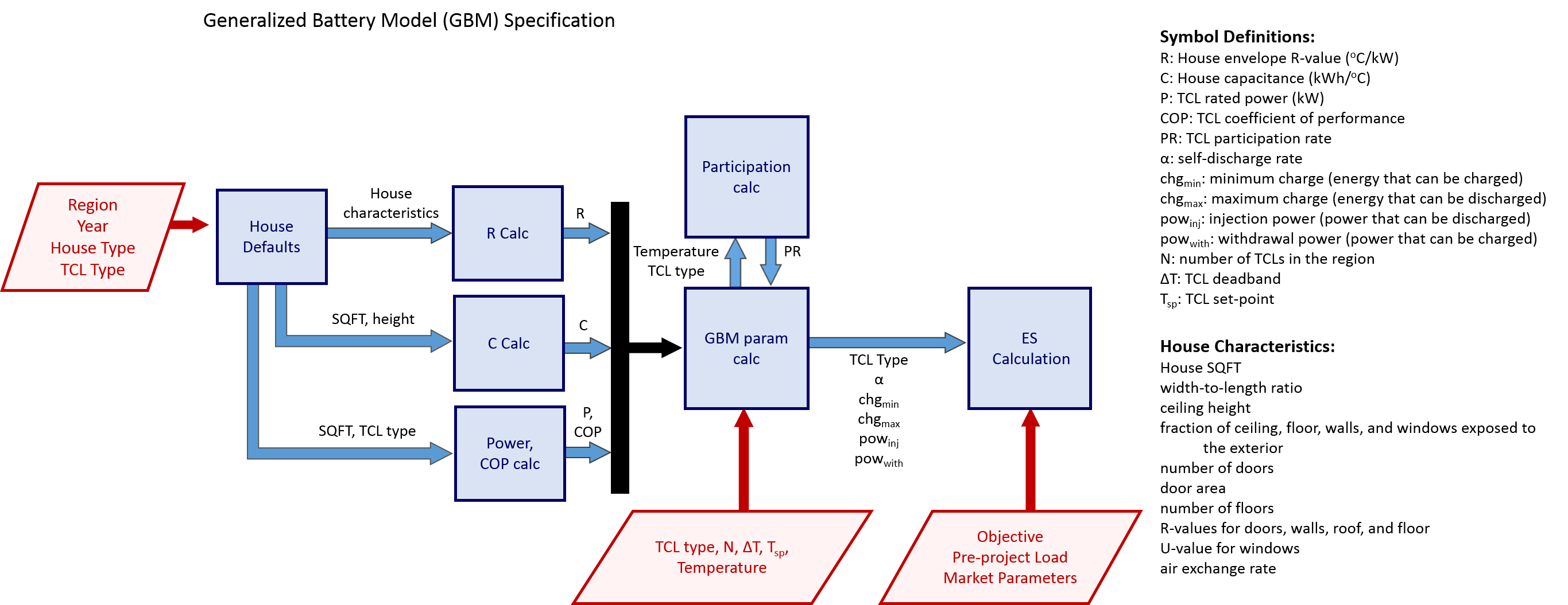
How GridPIQ Uses the GBM
The flowchart below illustrates how GridPIQ takes information about participating homes and equipment and uses it to model the behavior of a virtual battery. The housing and TCL inputs are used to calculate various thermal parameters, which in turn are inputs to the GBM parameter calculation. The GBM then defines the allowed behavior of the battery, which is used by the energy storage algorithm according to the project objectives. For more on how the thermal parameters are calculated, see this page. For a detailed description of the energy storage optimization routines, see the documentation for the market participation or peak shaving algorithms.
Deriving the GBM for Residential TCLs
Equivalent Thermal Parameter Model for a Single TCL
To transform demand response potential into energy storage, we begin with a simple first-order equivalent thermal parameter (ETP) model of a TCL, which describes the system in terms of a simple DC circuit. More information on how each TCL is modeled can be found here. In this formulation, temperature is analogous to voltage, the thermal conductance of a system’s envelope is equivalent to conductance (1/R), the thermal mass of a system is its capacitance (C), and heat flow is current. For air conditioning and heating, the system is the home itself, whereas for refrigeration or hot water heating, the system is an individual piece of equipment. For more information on the ETP model, see GridLAB-D documentation. For this model, the temperature \(\theta(t)\) in the space conditioned by the TCL is governed by
where \(s\) is a dimensionless binary variable indicating the operating state of the TCL and, for a cooling load, evolves according to
\( s(t+\epsilon) = \begin{cases} 0 & \theta(t+\epsilon) < \theta^s - \Delta \\ 1 & \theta(t+\epsilon) > \theta^s + \Delta \\ s(t) & otherwise \end{cases} \\\)where
\( \epsilon \ll 1 \): Small time increment
\(C\): Equivalent thermal capacitance of conditioned space
\(R\): Equivalent thermal resistance of conditioned space
\(P\): Rated power of TCL
\(COP\): Coefficient of performance of TCL
\(\theta^a(t)\): Ambient temperature surrounding conditioned space
\(\theta^s\): Set point temperature of TCL
\(\Delta\): Temperature deadband (user-specified allowable deviation from set point)
So, for example, if the cooling set point was 75oF with a deadband of 5oF, the AC would turn on above 80oF, turn off below 70oF, and remain in its current state between 70-80oF.
Extension to Multiple TCLs
To extend this model to many TCLs operating within a given region, we consider a continuous approximation of the ETP model above, which is accurate for a large population of TCLs [2]. The continuous model is given by
\( C \frac{d \theta(t)}{dt} = \frac{\theta^a(t) – \theta(t)}{R} – u(t) COP \\\) (5)
where \( u \) is the continuous power input from a population of TCLs; that is,
\( u(t) = \sum \limits_{i \in TCLs} u^i(t) \)
\( u^i(t) \in [0, P^i] \quad \forall i \in TCLs \)
Parameterization by Energy State
By making some substitutions, we can rearrange Equation 5 so that it is equivalent to the GBM charge-tracking constraint presented in Equation 4. If we define
\( x(t) = \frac{C}{COP} \left( \theta^s – \theta(t) \right) \): Battery charge at time t
\( p^{base}(t) = \frac{\theta^a(t) – \theta^s}{COP*R} \): Baseline power required to maintain the set point at time t
\( p(t) = u(t) – p^{base}(t) \): Net power into or out of the virtual battery
\( a = \frac{1}{RC} \)
then we obtain
\( \frac{d}{dt} \left( x(t) \right) = -a x(t) + p(t) \\\)which, when discretized into 1-hour increments indexed by \(t\), is equivalent to Equation 4:
\( X_{t+1} = \alpha X_t + P_t \Delta t \\\)where the self-discharge factor, \(\alpha = 1 – \frac{\Delta t}{RC}\), and \(\Delta t = 1 \).
Energy and Power Limits
The power limits for each hour are defined by the maximum possible deviation from the baseline power required to maintain the setpoint:
\( \overline{P}^{inj}_t = p^{base}_t \)
\( \overline{P}^{with}_t = P – p^{base}_t \\\)
The charge limits are defined as the amount of energy stored when the temperature deviates from its setpoint by the maximum permissible amount:
\( \overline{X}_t = \Delta \frac{C}{COP} \)
\( \underline{X}_t = -\Delta \frac{C}{COP} \\\)
Participation Factor
While the charge limits presented above appear time-independent, they do not account for variation in the number of devices available at each time step. Therefore, we modify the charge limits by a participation factor \(\nu\) that is a function of the ambient temperature. This factor accounts for the reality that at any given temperature, only some residential customers will be operating their HVAC systems. For example, if a typical AC set point is 75oF, few residents will have their ACs turned on at 70oF, but most will have them on at 100oF. We model this behavior with an inverse tangent function adapted from [2]. Refrigerators and water heaters are assumed to operate independent of temperature, but participation for ACs and heat pumps is determined by the following heuristic functions
Air Conditioners:
\( \nu_t^{AC} = \frac{\tan^{-1} \left( \theta^a_t – 27 \right) – \tan^{-1} \left( 20 – 27 \right)}{\tan^{-1} \left( 45 – 27 \right) – \tan^{-1} \left( 20 – 27 \right)}\)
Heat Pumps:
\( \nu_t^{HP} = 1 – \frac{\tan^{-1} \left( \theta^a_t – 10 \right) – \tan^{-1} \left( 0 – 10 \right)}{\tan^{-1} \left( 25 – 10 \right) – \tan^{-1} \left( 0 – 10 \right)}\)
The constants in the equations above determine the temperatures at which each device reaches 0, 50, and 100% participation. Sufficiently small (AC) or large (HP) values of \(\theta^a_t\) yield negative participation factors, which are simply replaced by zero.
After multiplying all charge and power limits by the corresponding participation factor, we have a fully constructed GBM ready to be operated by the energy storage optimization algorithms.
References
1. H. Hao, D. Wu, J. Lian and T. Yang, “Optimal Coordination of Building Loads and Energy Storage for Power Grid and End User Services,” in IEEE Transactions on Smart Grid. doi: 10.1109/TSG.2017.2655083
2. H. Hao, B. M. Sanandaji, K. Poolla and T. L. Vincent, “Aggregate Flexibility of Thermostatically Controlled Loads,” in IEEE Transactions on Power Systems, vol. 30, no. 1, pp. 189-198, Jan. 2015. doi: 10.1109/TPWRS.2014.2328865