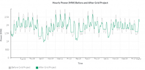
The daily peak reduction project assumes that a new energy storage system is operated to minimize load variance, which ultimately results in peak reduction and valley-filling. The figure below provides an example of the difference between the load profiles before and after the daily peak reduction energy storage project is applied.
The next figure provides a flow chart of the complete project module process flow.
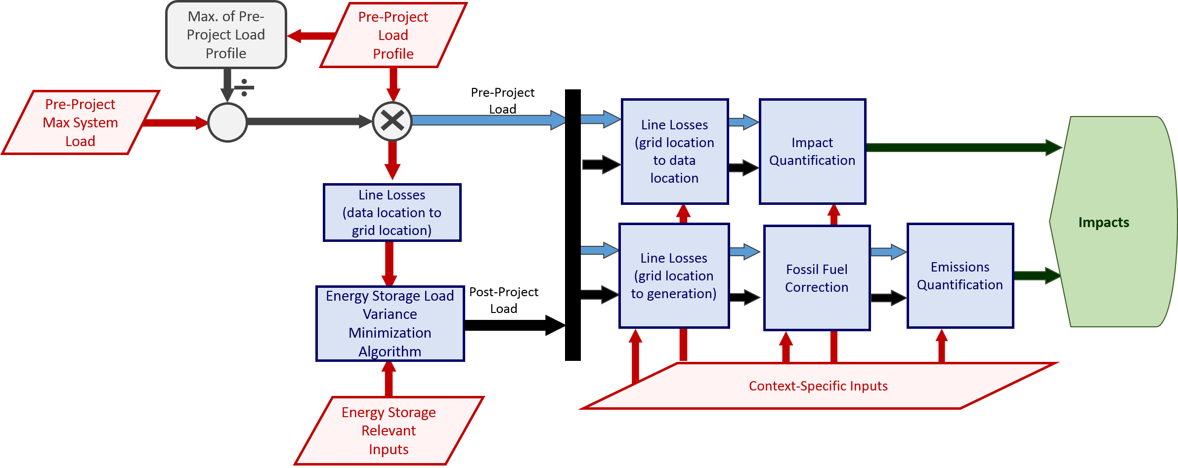
The energy storage load variance minimizaton algorithm is implemented with quadratic programming (QP) to minimize the cumulative quadratic of the load profile using the energy storage system over weeklong periods.
Energy Storage System Specifications
The specifications of any energy storage project generally include power and energy ratings. The power rating, specified here in megawatts (MW), determines the rate of transfer of energy that can be supplied or consumed per unit of time. A system with a higher power rating can charge or discharge quicker than one with a lower power rating. The energy capacity, specified in megawatt-hours (MWh), determines the total amount of energy that the system is able to store or deliver over time. The energy to power ratio (E/P) indicates the time duration (in hours, minutes or seconds) that the system can operate while delivering its rated output. For example, a lithium-ion battery with a power rating of 32MW, and an energy capacity of 8MWh, can deliver power for 15 minutes when discharging at its rated value.
The power and energy requirements may be different based on the target applications. If the primary function of the system is to provide frequency regulation, a higher power rating is preferred so that the system can charge and discharge frequently over a short duration of time. On the other hand, if the primary function is to enable peak-shifting or provide backup power in case of outage, the energy rating will be higher so that the battery can deliver power over a longer time.
Within the context of the optimization algorithm, operation of the energy storage project is constrained to ensure that its resulting discharge and charge behavior does not occur at a rate exceeding the power capacity defined by the user. Similarly, the user-supplied energy capacity dictates the maximum amount of energy that the system can store when it is fully charged. These values are provided by users in MW and MWh respectively.
The algorithm treats the energy capacity value as usable energy, assuming that the energy storage project can be discharged down to a 0% state of charge and charged to 100%, which may be different than system's nameplate capacity. As an example, if the storage system can only be operated between 20% and 100% of its nominal energy capacity, this value should be derated to 80% when entered it is into the calculator.
The round trip efficiency (RTE) of an energy storage project is defined as the ratio of the total energy output by the system to the total energy input to the system, as measured at the point of connection. The RTE varies widely for different storage technologies. A high value means that the incurred losses are low.
Algorithm Outputs
The ESS Daily Peak Reduction algorithm outputs a modified load profile, which can be used to quantify the project’s impacts based on its context.
Algorithm Description
The algorithm operates on the entire load period in discrete, weeklong segments with the first segment beginning at the first hour of the load profile. Any hours remaining at the end of the load profile are added to the final segment. We assume that the energy storage system (ESS) is fully charged when the optimizaton begins, and it is constrained to full charge at the end of each optimization period.
Optimization Routine Formulation
Variable definitions
\(p\): Power transfer between the ESS and the grid
\(p_{inj}\): Power injected into the grid by the ESS
\(p_{with}\): Power withdrawn from the grid by the ESS
\(P_{inj,max}\): Maximum ESS injection power
\(P_{with,max}\): Maximum ESS withdrawal power
\(eta^{+}\): Charge efficiency
\(eta^{-}\): Discharge efficiency
\(eta_{rt}\): Round-trip efficiency
\(E_{s}\): ESS energy capacity
\(SoC\): ESS state of charge
\(SoC_{min}\): Minimum ESS state of charge
\(SoC_{max}\): Maximum ESS state of charge
\(L\): Pre-project electrical load
\(K\): Total number of hours in the optimization period
Where:
\(p = p_{with} – p_{inj}\)
\(SoC_{k} = SoC_{k-1} + eta^{+} p_{with} – \frac{p_{inj}}{eta^{-}}\)
\(eta^{+} = eta^{-} = \sqrt{eta_{rt}}\)
In the implementation of the algorithm within the context of the website’s user interface, several additional assumptions are made. The charge and discharge efficiency values are assumed to be equal as well as the maximum charge and discharge powers. Additionally, the ESS is fully charged at the beginning of each optimization period and the algorithm enforces 100% state of charge at the end of the period. Finally, the minimum state of charge is zero and the maximum is the user-defined energy capacity.
\(P_{inj,max} = P_{with,max}\)
\(SoC_{1} = SoC_{K} = 1\)
\(SoC_{min} = 0\)
\(SoC_{max} = E_{s}\)
Objective function:
\(min[\sum (L + p)^{2}]\)
subject to:
Power injection limits: \(0 \leq p_{inj} \leq P_{inj,max}\)
Power withdrawal limits: \(0 \leq p_{with} \leq P_{with,max}\)
State of charge limits: \(SoC_{min} \leq SoC \leq SoC_{max}\)