GridPIQ draws hourly data reported to the EPA about the historical dispatch of fossil fuel plants, which is used to calculate emissions and fuel cost impacts. However, as most load profiles used in GridPIQ contain total electricity demand as served by all generation sources including non-fossil fuel resources, the relative hourly contributions of each type of fuel must be determined in order to properly calculate emissions resulting from operation of fossil fuel plants. These include plants that use coal, natural gas, oil, and other fuels derived from prehistoric organic matter.
Data Aggregation and Generation Dispatch Estimation Procedure
For each relevant analysis year, monthly electric power data has been obtained from the EIA’s Form 923. For each month in the analysis time period, electric power generation data for all electric generators with a nameplate capacity of 1MW or greater is used.
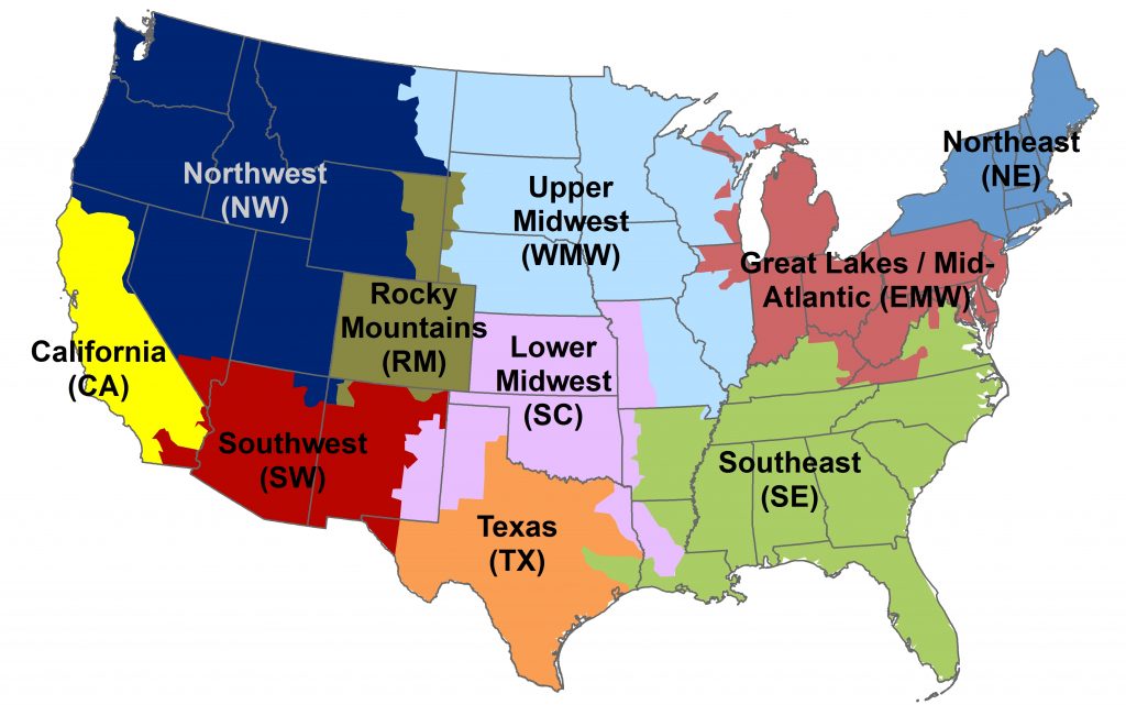
For each month, plant-level generation data is mapped to each of the AVERT regions using data from the EPA’s Emissions and Generation Resource Integrated Database (eGRID). AVERT regions are aggregations of eGRID subregions. The result of this mapping of power plant to AVERT region creates an approximate fuel mixture for each AVERT region for each month. Maps of the eGRID and AVERT regions can be found below.

Coupled with a classification system defining how generation types are assumed to operate within the system, this information is then used to estimate a likely dispatch order. The nine fuel types considered are grouped into four categories based on their operational characteristics, as illustrated in the table below.
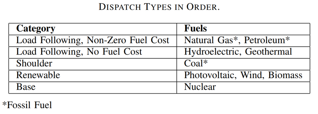
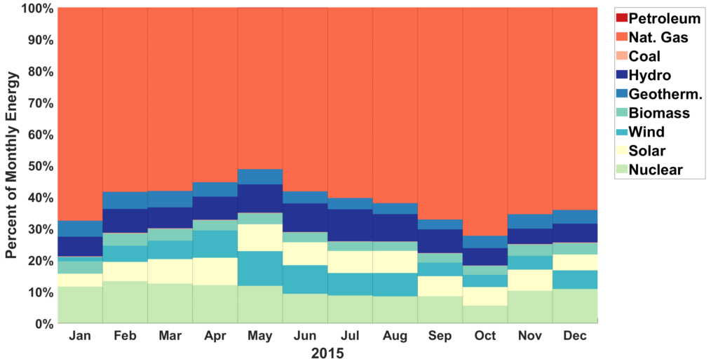
The four categories are given in order (top to bottom) from last deployed (peakers) to first deployed (base load). To construct a dispatch order for a month, each category of fuels is sorted based on the energy contribution by fuel for that month; the fuel that has the largest contribution within each operational category is assumed to be dispatched first, followed by the second largest, etc. The stack is thereby built from the bottom up category by category and fuel by fuel. An example of these stacks for the AVERT CA region in 2015 is illustrated below.
After determining monthly dispatch order and the percentage energy contributions by fuel type, it is possible to approximate how load is served for each hour of the month. The figure below illustrates GridPIQ’s estimation of dispatch for January 2015 in San Diego Gas & Electric’s (SDG&E) service territory. This example leverages load data pulled from the California Independent System Operator (CAISO) and typical meteorological year (TMY) data from the San Diego airport weather station to model wind and photovoltaic generation.
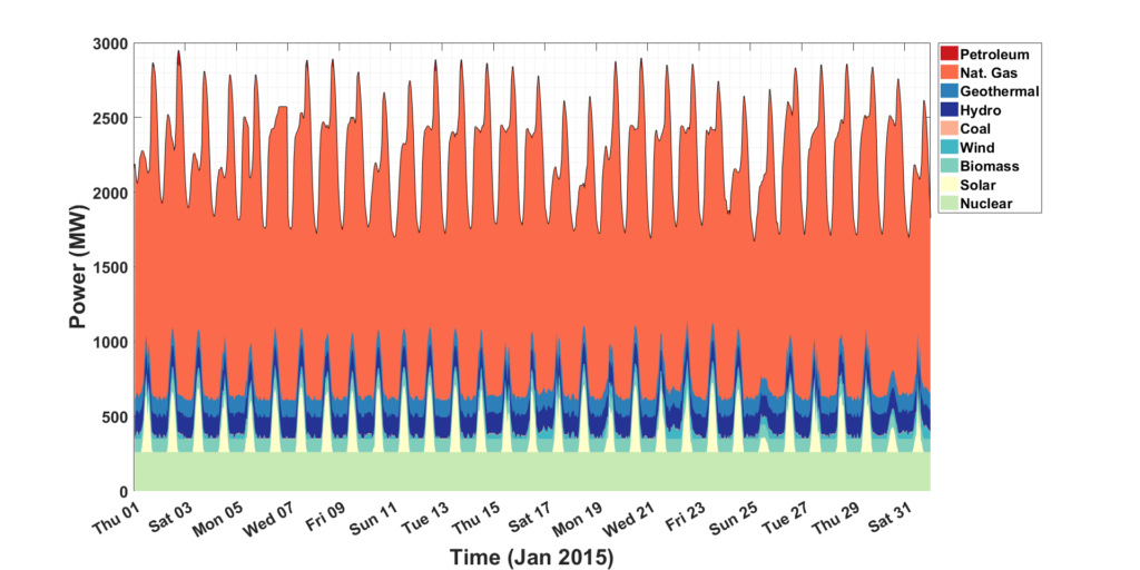
For each month, the pre-project load is combined with the regional fuel percentages, hourly wind and photovoltaic generation profiles, and dispatch order to compute the amount of load served by each fuel type for each hour. The percentage of load served by each fuel is set to match the regionally determined value. In the case of the variable, renewable resources, this is done by scaling the hourly profiles until their integral matches the requisite energy. In the case of the dispatchable resources (all but photovoltaic and wind), output is considered constant at a power output which results in the correct percentage of load being met, unless a constant output would cause generation to exceed load. If generation exceeds load, a binary search algorithm is used to find the power capacity for the given fuel so that its total energy generation matches the requisite percentage of energy served. The generators for this marginal fuel type will follow load up to the given power capacity. When that power capacity is exceeded, the next fuel in the stack is dispatched to meet additional demand.
For wind and photovoltaic generation, the energy contribution is described by the integral of hourly generation profiles, which represent the amount of load served by each resource in each hour. These profiles are created either with user uploaded time series data or TMY data from a user-selected weather station. If TMY data are used, the wind speed and direct horizontal irradiance are taken as an approximation of available resource for wind and photovoltaic generation, respectively. A first order model of wind turbine power output as a function of wind speed is used to create the wind power shape. When wind speed is below the cut-in speed, wind power output is assumed to be zero. Between the cut-in wind speed and the rated-power (or capacity) of the wind power generating resources, power output is modeled as a cubic of wind speed. Once the capacity of the generating resources is reached, power output is modeled as a cubic of the wind speed for which the generating resources are rated. In other words, the generating resources are assumed to be outputting their maximum capacity at this wind speed. In the model used here, maximum power output occurs at 13.86 m/s. Finally, above the cut-out speed, output is assumed to be zero. This is described mathematically below:
\(P(v) =
\begin{cases}
0 & v\leq 3.58 m/s \newline
v^3 & 3.58 m/s < v \leq 13.86 m/s \newline
13.86^3 & 13.86 m/s < v \leq 24.59 m/s \newline
0 & v > 24.59 m/s \newline
\end{cases}
\)
Where \(P\) is power output and \(v\) is wind speed in meters per second.
These wind-speed values are representative of a typical wind turbine according to an article released by the US Department of Energy. Note that this wind power model is not implemented for a user upload of wind power data, which is assumed to represent power output.
Regardless of where the hourly data comes from (user upload or TMY data), the time series profiles are scaled such that their total energy in the profile over the course of the month is equal to the generation type’s total energy contribution to the region. This is shown mathematically below.
\(\vec{y} = \frac{\vec{x}e_{tot}}{\sum_{n=1}^{H}x_{n}\Delta t} \)Where:
| Variable | Definition |
|---|---|
| \(\vec{y}\) | Vector representing the hourly average power output for the variable generating resource type in megawatts |
| \(\vec{x}\) | Vector either supplied by the user or derived from the TMY dataset representing either the expected generation profile or the approximate available resource |
| \(e_{tot}\) | Total energy contribution of the variable generating resource for the month under study in megawatt-hours |
| \(H\) | Number of hours in the month |
| \(\Delta t\) | Time interval in hours. GridPIQ operates only on hourly data, so this is always equal to one. |
Once the hourly generation profile for a fuel type has been created, it is applied to the load profile in the dispatch order determined by the tool. The full generation dispatch estimation procedure, including accounting for non-dispatchable generation, is best illustrated with an example.
Examine the SDG&E figure above for the month of January 2015, which shows the dispatch stack and fuel power contributions for each hour of the month as estimated by the tool. Note that the legend is arranged in dispatch order (read from the bottom up). The following subsections describe the procedure GridPIQ uses to determine dispatch.
Nuclear
As a “Base” category fuel type, nuclear generation is at the bottom of the dispatch stack, meaning that it will be deployed first to serve load. Because nuclear is a dispatchable resource with capacity below the power demand all month, it is modeled as operating at a constant output level throughout the month, making the maximum power level for nuclear generation its total energy contribution for the month divided by the number of hours in the month. The remaining generating resources must serve the original load profile minus the nuclear contribution.
Photovoltaics
In this example, the next generation type in the dispatch order is photovoltaics. Because photovoltaic generation is a variable, non-dispatchable resource, the scaled hourly generation profile is used rather than assuming a flat generation profile. Recall that in this example, TMY solar irradiation data from the San Diego airport is used to approximate the shape of the photovoltaic generation profile. This scaled profile serves as much of the remaining load as possible, reducing that which must be met by the remaining generation types. In most scenarios, this will be all that’s required to account for the contribution of photovoltaic generation to the region’s energy mix.
However, sometimes, subtracting the solar generation profile causes the remaining load profile to dip below zero, requiring an additional step. Given that the fuel mixture percentages for the given region represent regional load served by generation type and that this methodology assumes that generation types lower in the stack (i.e. nuclear) will not be curtailed during hours of high renewable penetration, the tool constrains the maximum photovoltaic output at any given hour to the amount of unserved load within that hour. In other words, the tool crops any hours of photovoltaic generation that would cause load to become negative and then accounts for this reduced overall photovoltaic generation by scaling all other hours of photovoltaic output up so that the total monthly energy served by photovoltaics still matches the regional percentage.
Biomass
Next in the dispatch order is biomass in this instance. At this point in the process, both nuclear and photovoltaic generation have been accounted for and subtracted from the load profile. In this example, biomass meets approximately 4% of the energy for the month and biomass is assumed to operate at a constant power output for the entire month because a flat profile does not exceed demand for any hour.
Wind
Wind, like photovoltaic generation, is non-dispatchable so a profile is used that varies hourly, in this case scaled TMY wind speed data from the San Diego airport. The procedure for scaling and cropping if necessary is identical to that described in the photovoltaics section above.
Coal, Hydro, and Geothermal
In this example, coal, hydroelectric, and geothermal generation are all dispatchable and act as constant baseload for this profile, just as nuclear and biomass did, following the same procedure.
Natural Gas
In this case, natural gas is the primary load following generation resource. A binary search algorithm is used to determine its power capacity such that natural gas meets the prescribed percentage of demand in every hour.
Petroleum
Though not visible in the figure, petroleum-fired generation units are used to meet peaks in demand that exceed natural gas’s determined capacity. In this example, petroleum generation accounts for less than 1% of energy served. The section below presents another example with more petroleum generation.
Calculating the Fossil-Fuel Portion of the Load Profile
After hourly dispatch has been determined for each month, the pre-project load profile is corrected to represent only load that is served by fossil fuels. As alluded to above, this simply involves hourly subtraction of demand met by non-fossil fuels from the load profile, or equivalently adding up those met by fossil fuels.
Note that the fuel power capacity values and renewable profiles are determined for the pre-project load profile, and the same values and profiles are used for estimating generation dispatch for the post-project load profile. If the post-project load profile is dramatically different from the pre-project load profile, errors can be introduced. Specifically, if the peak in the post-project load profile is larger than the peak in the pre-project load profile, this will result in a “stretching” of the contribution of the resource highest in the dispatch stack. In other words, whichever fuel is on the top of the stack is assumed to ramp up to meet additional demand. Conversely, imagine a project which results in peak shaving and valley filling (like GridPIQ’s Energy Storage for Daily Peak Reduction project). If peak demand is shifted so that it is served by a different fuel, the fuel at the top of the stack will serve less load that month, and the fuel in the “valley” will serve more.
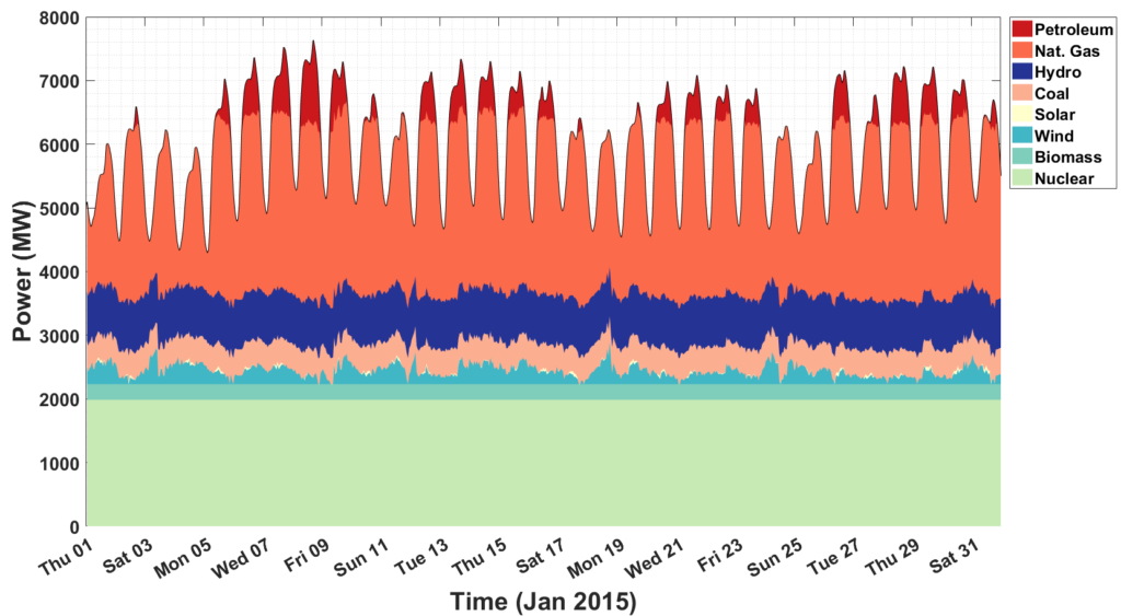
Another Example
The figure below depicts GridPIQ’s hourly dispatch approximation for a load profile for New York City (NYC) from the New York Independent System Operator (NYISO). In this case, TMY data from JFK airport is used. Notice that both natural gas and petroleum are performing load following duties, and that photovoltaic generation serves a much smaller portion of demand than in the previous example.